[NOTE] Kaggle house price prediction
Abstracts
This is a copycat of Comprehensive data explorationi with Python. Since I had limited time to accomplish AI project. So I preferred learn from other’s notebook. And ‘Comprehensive data explorationi with Python’ is apparently the most fit one for me.
According to the article, the first thing we should do is look through the whole data set, and find the most important variables which matters when you buy a house.
And then an important problem we must deal with is Data Cleaning.
Overviews
While ‘Type’ and ‘Segment’ is just for possible future reference, the column ‘Expectation’ is important because it will help us develop a ‘sixth sense’. To fill this column, we should read the description of all the variables and, one by one, ask ourselves:
- Do we think about this variable when we are buying a house? (e.g. When we think about the house of our dreams, do we care about its ‘Masonry veneer type’?).
- If so, how important would this variable be? (e.g. What is the impact of having ‘Excellent’ material on the exterior instead of ‘Poor’? And of having ‘Excellent’ instead of ‘Good’?).
- Is this information already described in any other variable? (e.g. If ‘LandContour’ gives the flatness of the property, do we really need to know the ‘LandSlope’?).
I went through this process and concluded that the following variables can play an important role in this problem:
- OverallQual 总体质量
- YearBuilt.
- TotalBsmtSF. 地下室面积
- GrLivArea. 地上居住面积
Hmmm… It seems that ‘SalePrice’ and ‘GrLivArea’ are really old friends, with a *linear relationship.***
In my opinion, this heatmap is the best way to get a quick overview of our ‘plasma soup’ and its relationships. (Thank you @seaborn!)
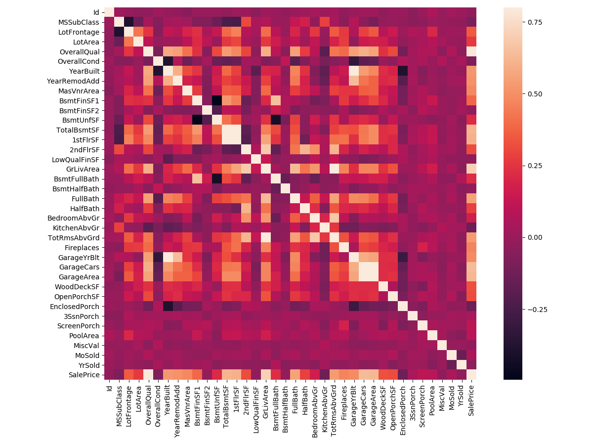
- TotalBsmtSF and 1stFlrSF
- GarageX
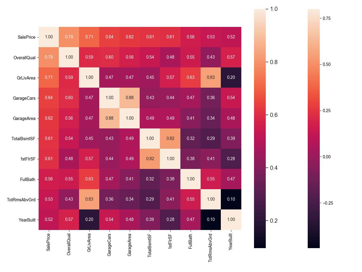
According to our crystal ball, these are the variables most correlated with ‘SalePrice’. My thoughts on this:
- ‘OverallQual’, ‘GrLivArea’ and ‘TotalBsmtSF’ are strongly correlated with ‘SalePrice’. Check!
- ‘GarageCars’ and ‘GarageArea’ are also some of the most strongly correlated variables. However, as we discussed in the last sub-point, the number of cars that fit into the garage is a consequence of the garage area. ‘GarageCars’ and ‘GarageArea’ are like twin brothers. You’ll never be able to distinguish them. Therefore, we just need one of these variables in our analysis (we can keep ‘GarageCars’ since its correlation with ‘SalePrice’ is higher).
- ‘TotalBsmtSF’ and ‘1stFloor’ also seem to be twin brothers. We can keep ‘TotalBsmtSF’ just to say that our first guess was right (re-read ‘So… What can we expect?’).
- ‘FullBath’?? Really?
- ‘TotRmsAbvGrd’ and ‘GrLivArea’, twin brothers again. Is this dataset from Chernobyl?
- Ah… ‘YearBuilt’… It seems that ‘YearBuilt’ is slightly correlated with ‘SalePrice’. Honestly, it scares me to think about ‘YearBuilt’ because I start feeling that we should do a little bit of time-series analysis to get this right. I’ll leave this as a homework for you.
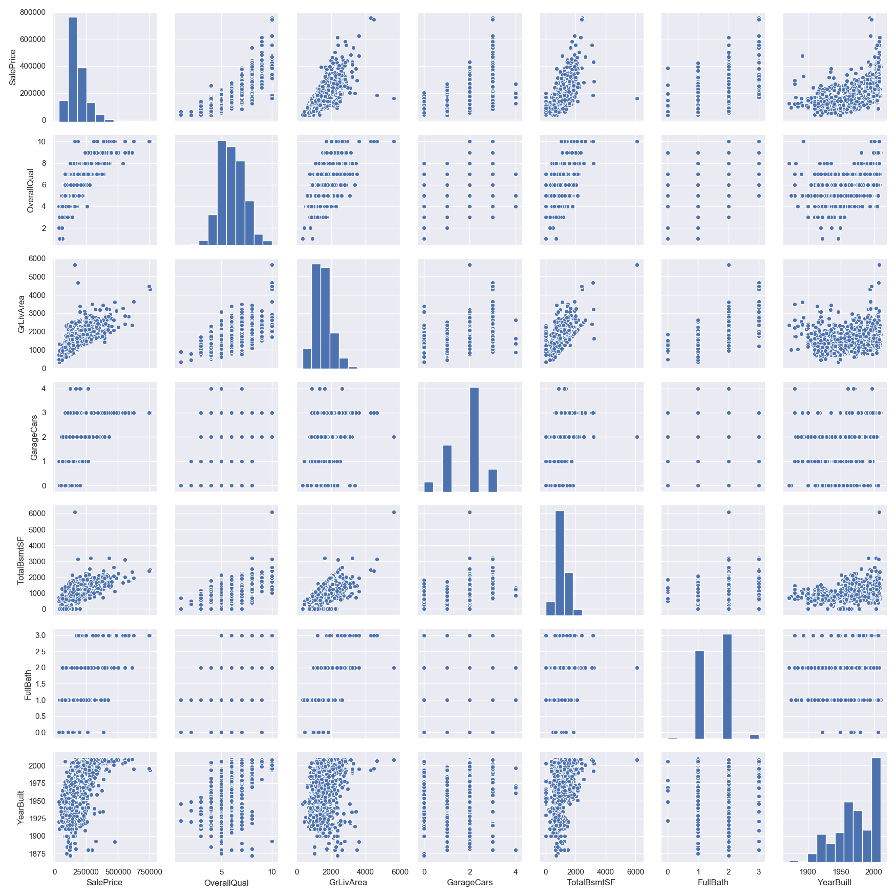
Let’s proceed to the scatter plots.
Missing data
Missing data analysis
Using script below, we can easily get the missing data.
1 | #missing data |
| Total | Percent | |
|---|---|---|
| PoolQC | 1453 | 0.995205 |
| MiscFeature | 1406 | 0.963014 |
| Alley | 1369 | 0.937671 |
| Fence | 1179 | 0.807534 |
| FireplaceQu | 690 | 0.472603 |
| LotFrontage | 259 | 0.177397 |
| GarageCond | 81 | 0.055479 |
| GarageType | 81 | 0.055479 |
| GarageYrBlt | 81 | 0.055479 |
| GarageFinish | 81 | 0.055479 |
| GarageQual | 81 | 0.055479 |
| BsmtExposure | 38 | 0.026027 |
| BsmtFinType2 | 38 | 0.026027 |
| BsmtFinType1 | 37 | 0.025342 |
| BsmtCond | 37 | 0.025342 |
| BsmtQual | 37 | 0.025342 |
| MasVnrArea | 8 | 0.005479 |
| MasVnrType | 8 | 0.005479 |
| Electrical | 1 | 0.000685 |
| Utilities | 0 | 0.000000 |
So how to handle the missing data?
We’ll consider that when more than 15% of the data is missing, we should delete the corresponding variable and pretend it never existed. So we delete ‘PoolQC’, ‘MiscFeature’, ‘Alley’, ‘Fence’, ‘FireplaceQu’ and ‘LotFrontage’.
As for ‘GarageX’, they all have the same number of missing data. Maybe the missing data refers to the same set of observations. Since the most important information regarding garages is expressed by ‘GarageCars’ and considering that we are just talking about 5% of missing data, I’ll delete the mentioned ‘GarageX‘ variables. The same logic applies to ‘BsmtX‘ variables.
As for ‘MasVnrArea’(砖石饰面面积) and ‘MasVnrType’(砖石饰面种类), we can consider that these variables have a strong correlation with ‘YearBuilt’ and ‘OverallQual’ which are already considered. So we delete ‘MasVnrArea’ and ‘MasVnrType’.
Delete missing variables
We’ll delete all the variables with missing data, except the variable ‘Electrical’. In ‘Electrical’ we’ll just delete the observation with missing data.
1 | #dealing with missing data |
If the output is ‘0’, it means you have fully delete missing data.
Out liars
The primary concern here is to establish a threshold that defines an observation as an outlier. To do so, we’ll standardize the data. In this context, data standardization means converting data values to have mean of 0 and a standard deviation of 1.
1 | 这里主要关注的是建立一个将观察值定义为异常值的阈值。为此,我们将对数据进行标准化。在这种情况下,数据标准化意味着将数据值转换为平均值为0且标准差为1。 |
1 | #standardizing data |
这一步的目的应该是为了找出数据中的离群值,这里需要关注的是两个大于7的变量。
1 | #bivariate analysis saleprice/grlivarea |
将’GrlivArea’中的离群值删除。
之后考察’TotalBsmtSF’中的离群值,但它的离群值表现在可以接受的范围之内。
Getting hard core
According to Hair et al. (2013), four assumptions should be tested:
- Normality: The data should look like a normal distribution.
- Homoscedasticity: 这个用英文解释不太好懂,同方性是可取的,我们希望误差项在自变量的所有值上都相同;
- Linearity: 正如前文已经做过的,通过散点图的方法来观测两个变量之间是否有线性的相关性,如果相关性不是线性的,那么可以通过一定的数学转换使其线性相关;
- Absence of correlated errors:
Normality
The point here is to test ‘SalePrice’ in a very lean way. We’ll do this paying attention to:
- Histogram - Kurtosis and skewness.
- Normal probability plot - Data distribution sould closely follow the diagonal that represents the normal distribution.
1 | #histogram and normal probability plot |
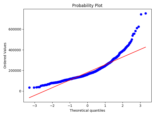
对变量取log转换得:
1 | #applying log transformation |
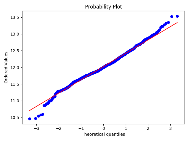
可以看到,散点更为均匀地分布在了直线的两侧。
以同样的方法对’GrLivArea’与’TotalBsmtSF’进行处理。
其中面临一个很严重的问题是,有些值为0,所以在这些值上,我们无法对它们取log。要在此处应用对数转换,我们将创建一个变量,该变量可以具有或不具有地下室的效果(二进制变量)。然后,我们将对所有非零观测值进行对数转换,而忽略那些值为零的观测值。这样,我们可以转换数据,而不会失去某些变量的影响。
1 | #create column for new variable (one is enough because it's a binary categorical feature) |
Main Variables
| Variable | Segment | Data Type | Comments |
|---|---|---|---|
| GrLivArea | 1 | 0 | 生活面积 |
| TotalBsmtSF | 1 | 0 | 地下室总面积 |
| GarageArea/GarageCars | 1 | 0 | 车库 |
| YearBuilt | 0 | 1 | 建造年份 |
| CentralAir | 0 | 1 | 中央空调 |
| OverallQual | 0 | 1 | 总体评价 |
| Neighborhood | 2 | 1 | 地段 |
Now we can make sure there 7 variables will participate in our model. And we have cleaned the data set. The final thing left to do is to get the PREDICTION.
Model: Random forest
Why use this? Idk, otherwise the blog didn’t describe the reason clearly.
The code displays below. And I have little trouble understanding the Random Forest Algorithm.
1 | # 获取数据 |